How does logistic regression work in Python. This is the story.
We are going to look into the theory and application of logistic regression. This story will follow the outline of the course from lazy programmer here: https://lazyprogrammer.me/deep-learning-courses/.
Theory
We are still using the formula for from linear regression \(y=ax+b\), but in machine learning we often use different wording than what we typically do in statistics.
The constant term is renamed to \(w_1\) and the bias/intercept to \(w_0\), so we get:
making h() a linear combination of the components of x. In vector form we write \(h(\textbf{x})=\textbf{w}^t\textbf{x}\)
Calculate the output of a neuron
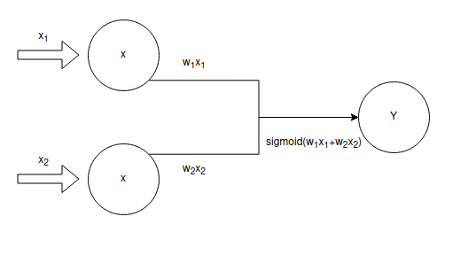
The sigmoid function we will use: \(\sigma(z) = \frac{1} {{1+e^{-z}}}, \in{(0,1)}\), which can be written as: \(\sigma(\textbf{w}^t\textbf{x})\)
To do the logistic regression in Python, we do this:
import numpy as np

N = 100
D = 2

X = np.random.randn(N, D)  # The dataset
ones = np.array([[1]*N]).T  # the bias/intercept
Xb = np.concatenate((ones, X), axis=1)  # just the dataset as a N x 3 matrix

w = np.random.randn(D + 1)  # weights, must be a 3 x 1 matrix

# Calculate the dot product between x and w
z = Xb.dot(w)  # Will be a (Nx3) * (3x1) = N x 1 matrix

def sigmoid(z):
    return 1 / (1 + np.exp(-z))

print(sigmoid(z))
Example with ecommerce data
Example data
The data looks something like this:
import numpy as np
import pandas as pd

df = pd.read_csv('ecommerce_data.csv')
df.head()
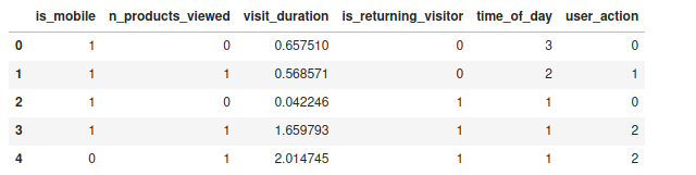
The 'visit_duration' is a real number in minutes of how long the user was on the site.
'time_of_day" is a category label:
0: from 0 to 6
1: from 6 to 12
2: from 12 to 18
3: from 18 to 24
We will do 'one hot encoding' for this category:
| 0-6 / | 6-12 / | 12-18 / | 18-24 |
|---|---|---|---|
| 1 | 0 | 0 | 0 |
| 0 | 1 | 0 | 0 |
| 0 | 0 | 1 | 0 |
| 0 | 0 | 0 | 1 |
User action is the action we want to predict:
0: bounce
1: add_to_cart
2: begin_checkout
3: finish_checkout
Normalize
Scale and distance are important so we need to normalize the n_products_viewed and the visitor_duration numbers, which can be done according to the formula \(Z= \frac{(X-\mu)} {\sigma}\)
Pre-process data
Normalize numerical columns
We have 2 numerical columns that we want to normalize, the first and second ones. We will create a function to do this:
def normalize_row(row):
    """Takes a row and returns a normalized row"""
    return (row - row.mean()) / row.std()
We then create a new X matrix with the first 2 rows normalized:
data = df.to_numpy()  # makes the dataframe into a numpy array

X = data[:, :-1]  # All the X variables
Y = data[:, -1]  # The dependent Y variable

# Normalize rows 1 and 2 in place
X[:,1] = normalize_row(X[:,1])
X[:,2] = normalize_row(X[:,2])
The we do the one how encoding for the time dimension:
## The 'time of day' category column. We want to use the one-hot encoding.
N, D = X.shape  # D = 5 as there are 5 columns in X
X2 = np.zeros((N, D+3))  # D + 3 = 5 + 3=8; We will have the existing 4 categories + 4 'one hot encodings' for the 'time_of_day' column
X2[:, 0:(D-1)] = X[:, 0:(D-1)]  # X2's first 4 columns just contains the original 4 X columns

# The one hot encoding
for n in range(N):
    time_of_day = int(X[n, D-1])  # D-1=4, the 4th column in the original X matrix is the 'time_of_day' column (we count from zero)
    X2[n,time_of_day + D-1] = 1  # time_of_day + (D-1) = the category used in the one hot encoding; and we set that == 1
Additionally, in logistic regression, we are only operating with 2 'categories' for the dependent variable (Y), in our case 'bounce' or 'add_to_card', which have values 0 and 1 respectively. We filter our X2 and Y variable to only include rows with these two Y categories:
X2 = X[Y <=1 ]
Y = Y[Y <= 1]
Make prediction
We start by creating the weights and bias for our predictive model. The weights will initially just be random numbers and the bias is set to zero:
D = X2.shape[1]  # Getting the number of columns in our X2. We will use this to create our initial weights
W = np.random.randn(D)  # Our weights matrix, just random numbers
b = 0  # Bias term.
We will create 2 helper functions to assist us with our prediction, a sigmoid function and a prediction function.
Sigmoid function
def sigmoid(a):
    return 1/(1 + np.exp(-a))
Prediction function
def forward(X, W, b):
    return sigmoid(X.dot(W) + b)
We make the prediction:
P_Y_given_X = forward(X, W, b)
predictions = np.round(P_Y_given_X)
The classification rate function:
def classification_rate(Y, P):
    return np.mean(Y == P)
Running all this, we can get something like this (depending on your random weights):
print("Score:", classification_rate(Y, predictions))
Score: 0.30402010050251255
Training and solving for optimal weights
The cross entropy error function
What do we want out of an error function for a logistic error function: * Should be 0 if there is no error * > 0 if there is an error * Magnitude means higher cost
The cross-entropy error function is:
Where:
J: is the error
t: is the target
y: is the prediction, or the output from the logistic regression
Lets try and set t = 1:
So only the first term really matter in this case. If we set t=0, we get:
So only the 2nd term matter.
If we try a few examples this might make more sense.
With t=1 and y=1 (our real value (target) was 1 and the prediction was also one), then our error becomes:
Which intuitively makes sense, we hit the target so the error becomes zero. The same thing happens if we have t=0 and y = 0.
What if our prediction is just a bit off? say t=1 but y=0.9? Then we get:
So a relatively small error.
What if we have a large difference between t and y, say t = 1 and y = 0.2?
Giving us a much larger error.
For the calculations we typically want the total cross entropy error which we get by summing over all the errors:
Making a function
We are gonna make use of the fact that the cross entropy error function simplifies for t = 0 and t = 1. We can then do this:
def cross_entropy_error(T, Y):
    """Calculate the cross entropy error.
    T: Target
    Y: Prediction
    """
    N = T.shape[0]
    E = 0
    for i in range(N):
        if T[i] == 1:
            E -= np.log(Y[i])
        else:
            E -= np.log(1 - Y[i])

    return E
Calculation example in code
N = 100
D = 2

X = np.random.randn(N, D)  # Random Xs with same mean and variance

X[:50, :] = X[:50, :] - 2 * np.ones((50, D))  # make half 2*1 lower than mean
X[50:, :] = X[50:, :] + 2 * np.ones((50, D))  # make other half 2*1 higher than mean

T = np.array([0] * 50 + [1] * 50)  # Target, first 50 are 50 then next 50 one.

# Create X matrix with constants term
ones = np.array([[1] * N]).T
Xb = np.concatenate((ones, X), axis=1)

# Randomly initialize the weights
w = np.random.randn(D + 1)

# Calculate model output
z = Xb.dot(w)
Y = sigmoid(z)

print(cross_entropy_error(T, Y))
158.89255979864652
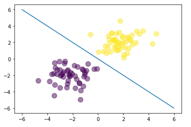
Let's try and visualize this solution. We first import matplotlib:`
import matplotlib.pyplot as plt

# The closed form solution
w = np.array([0, 4, 4])  # bias is zero

# The line: y = -x
plt.scatter(X[:,0], X[:,1], c=T, s=100, alpha=0.5)  # c=T for the colors
x_axis = np.linspace(-6, 6, 100)
y_axis = -x_axis
plt.plot(x_axis, y_axis)
plt.show()
Cross entropy error and log likelyhood
An interesting consequense of having the cross entropy error function the way we have it is that maximizing the log likelihood of our sigmoid function is the same as minimizing the cross entropy error function.
(Will not show the math here though)
Gradient decent
Theory
The basic idea of gradient decent is that we take small steps in the direction of the derivative. So we update our weights with a small step size (choosen by us) and rerun until our derivative is so close to zero as we are comfortable with.
How to choose the learning rate? No scientific way, just try.
The derivative becomes:
The derivative of the sigmoid becomes:
The deriviative of a with respect to w (the activation with regards to the weights):
Putting it all together:
In vector form:
In code
N = 100
D = 2

X = np.random.randn(N, D)  # Random Xs with same mean and variance

X[:50, :] = X[:50, :] - 2 * np.ones((50, D))  # make half 2*1 lower than mean
X[50:, :] = X[50:, :] + 2 * np.ones((50, D))  # make other half 2*1 higher than mean

T = np.array([0] * 50 + [1] * 50)  # Target, first 50 are 50 then next 50 one.

# Create X matrix with constants term
ones = np.array([[1] * N]).T
Xb = np.concatenate((ones, X), axis=1)

# Randomly initialize the weights
w = np.random.randn(D + 1)

# Calculate model output
z = Xb.dot(w)
Y = sigmoid(z)

learning_rate = 0.1
# Do 100 iterations of gradient decent
for i in range(100):
    if i % 10 == 0:
        ce_error = cross_entropy_error(T, Y)
        print(f"Cross entropy error: {ce_error}")

    w += learning_rate * np.dot((T - Y).T, Xb)
    Y = sigmoid(Xb.dot(w))


print(f"Final w: {w}")